Introduction

In the early 1960s the use of computers was via BATCH processing where a computer user submitted a computer task via a Paper Tape or a deck of Punch Cards to computer operators who ran the jobs through the computer in batches. Several jobs were read to magnetic tape to create an input tape. The input tape was read as the input to the batch process, magnetic tape being a hundred times faster than paper tape or punch cards which were electro-mechanical devices. If the computer had read the jobs directly it would have been idle for 90% of the time awaiting input. The output was written to magnetic tape to create an output tape. This tape was printed out whilst other jobs were being read in to create another input tape whilst the 2nd input tape jobs were being processed. The user was meantime doing other things. The results of the job would come hours later or next day.

In the early 1960's people had a vision of reacting directly with the computer via a device called a 'terminal'. The terminal was a typewriter-like device, with a keyboard and a fan-folded strip of paper with sprocket holes each side, fed over a platen. Commands were typed, printed on the paper and read by the computer. When the carriage return was pressed the computer obeyed the command and printed back the result. Commands would be entered and a response received within milliseconds, generally an error message, when the user could invoke an editor to correct their program and resubmit it.

This process of coding, compiling, running, error message, editing, compiling, running, ... might go on for a short time for a clever programmer, or for ever for a bad programmer.

Terminals were located close to the computer user, not in their office but in a room close by. The terminals would be shared by several users. Each terminal was connected to a communications controller in the computer room. Terminals on the University Campus were connected via a 4 core screened cable. Terminals off-campus had to be connected via the General Post Office private wires.

This was 1971 when both the Postal Service and the Telephone Service were one organisation, it was split in 1980 when the telephone service was privatised and became British Telecom. This document listed the GPO telephone lines: both private wires and exchange connections. When something stopped working we had to check our own equipment before phoning the GPO to report a line fault. We needed to specify the 'Line #' which we found from this diagram. I remember we used to dial 151. Looking now in 2012 the number to dial is 0800 800 151, but just now I tried dialing 151 and it connects to the same 0800 800 151 service 41 years later.

This first network diagram is as simple as you can get.

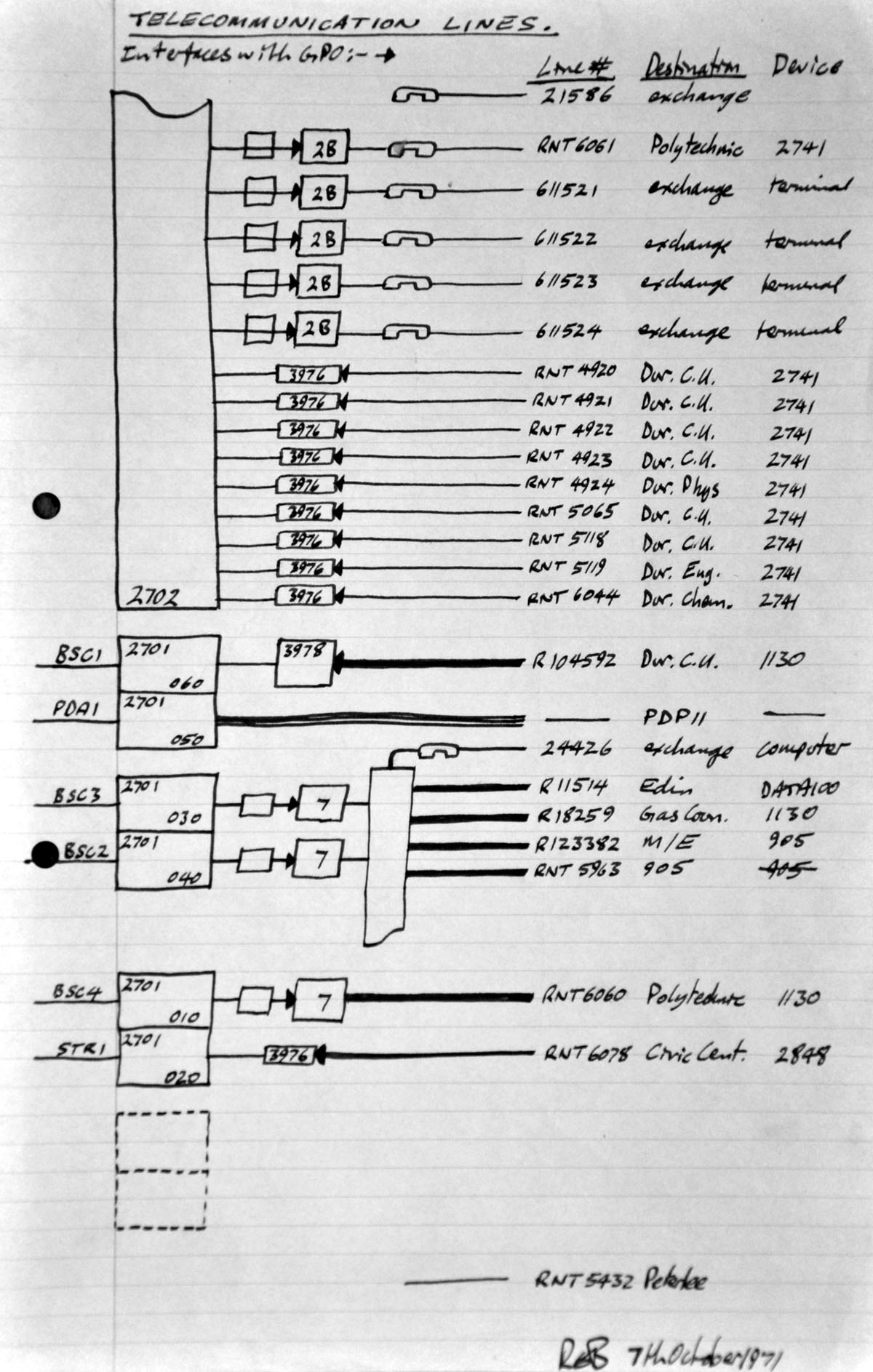
It is just a list of telephone lines connecting remote terminals and computers.

On the left are boxes labelled "2701" and "2702". These were communication controllers connected to the mainframe computer that contained devices which information could be written to or read from. To these devices modems were connected, to which were connected private telephone wires. These private wires were 4 copper conducters, 2 transmit, 2 receive, that went through underground ducts, junction boxes, telephone exchanges, to the destination where there was another modem connected to the remote equipment. The two modems were synchronised to each other by each transmitting a carrier signal. A digital signal from the communications device was modulated on the carrier signal and the remote modem demodulated it to reconstruct the original digital signal.

There were two types of modem: slow ones "2B" "3976" operating at 200bps and fast ones "7" "3978" operating at 9600bps. Here is a 200bps modem and here a 9600bps modem.

The destinations were
21586 exchange - a GPO telephone exchange line. This was the external telephone line to the Computer Operators.
RNT6061 Polytechnic private wire to Newcastle Polytechnic connected to an IBM 2741 terminal.
The next four were exchange lines connected to 2B modems which remote users with terminals connected to compatible modems could dial to and make a data connection.
The next 9 beginning RNT... Dur.C.U. were private wires connected to IBM 3976 modems. Phys and chem and ... were remote places.

There were other terminals, not listed here, because they directly connected on campus via 4 core screened cables belonging to the university.

The "REB 7th October 1971" at the bottom is me Roger Edward Broughton signing the document.

This next document listed the GPO equipment connected to the IBM 360/67 computer in 1972, the number of lines and annual rental. It is similar to 1971 in that there are 30 private wires, just 4 more. There is just speed, no line identification, and cost per annum.

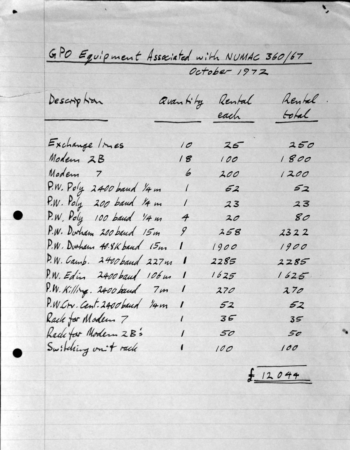
The annual rental was a combination of distance and speed.

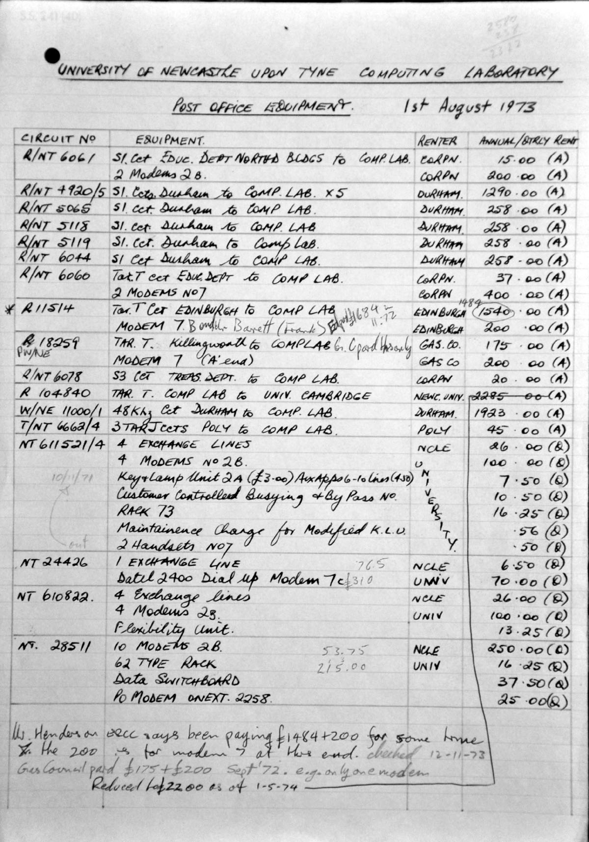
A year later in 1973 up to 32 telephone lines. Here is a more interesting document giving:
The CIRCUIT No, EQUIPMENT, RENTER, and ANNUAL/QTRLY RENT.

Although not a network as we would understand it, the terminal connections to mainframe computers at DURHAM, EDINBURGH and CAMRIDGE would have not only enabled access to those computers that might have data, software packages that were not locally available at Newcastle but, also onward connection to computers connected to those computers. This was the beginning of a global network.

Two years later in 1975 the first NUNET node was added, by 1977 there were 4 nodes in other buildings, each node connecting several terminals to the IBM 370/168, the memory of which had been increased by 4Mb of EMM memory.

In 1979 NUNET supported 200 terminals, some of them were computer terminals capable of supporting local visual editing. Greater than 150 interactive terminals was too much for MTS to support.

In 1983 there was a connection to JANET (Joint Academic Network). JANET was a WAN (Wide Area Network) connecting LANs (Local Area Networks) in academic and research institutions over the whole of the UK.

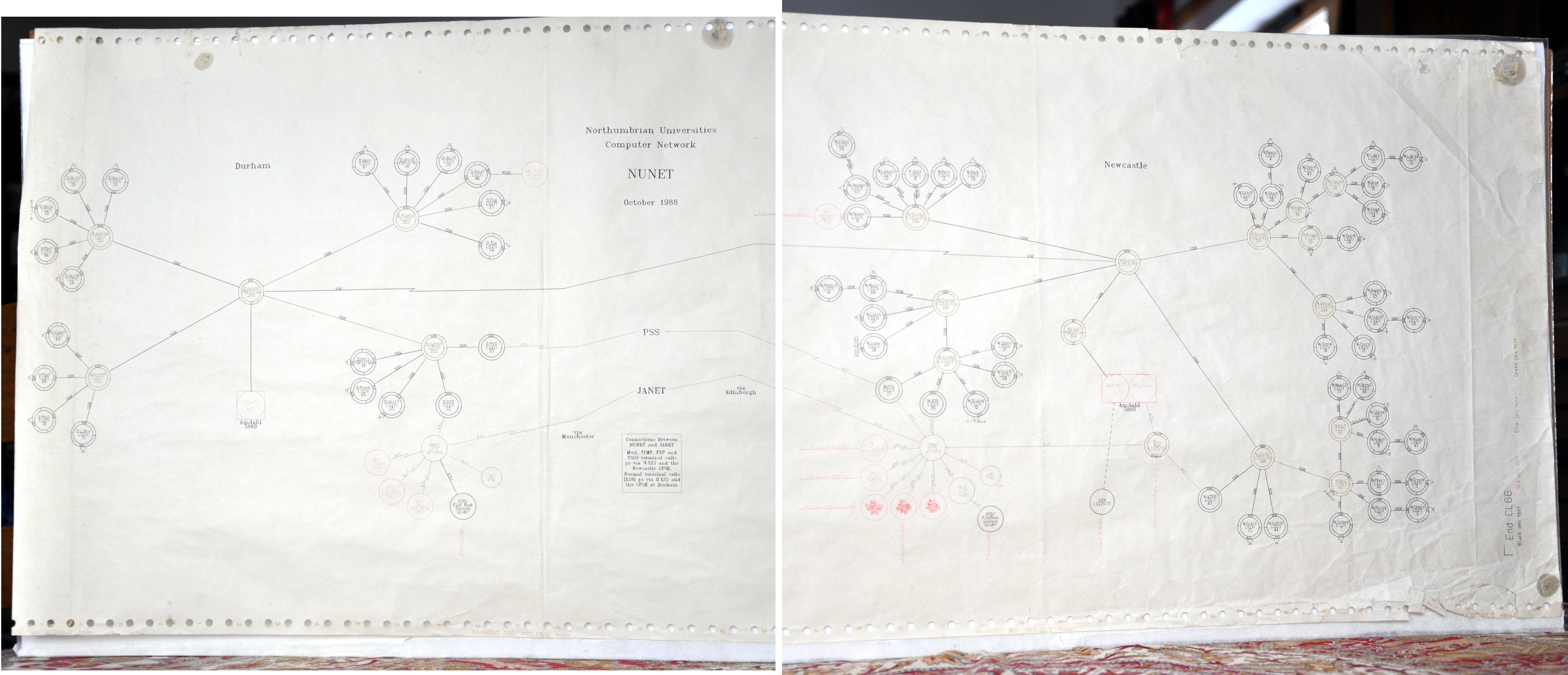
Here is a network diagram from 1985. It is the first year of the last mainframe, the Amdahl 5860, red circle left of the top middle pair. Also new was the Amdahl 470/V8 at Durham, right of top middle pair.

Other red circles are scattered around the network. The 12 at Newcastle and 3 at Durham are other computers augmenting the mainframe service. Over the next seven years all of the services would be unpacked from the mainframes and be distributed to suitcase-sized machines, each having a keyboard and a monitor.

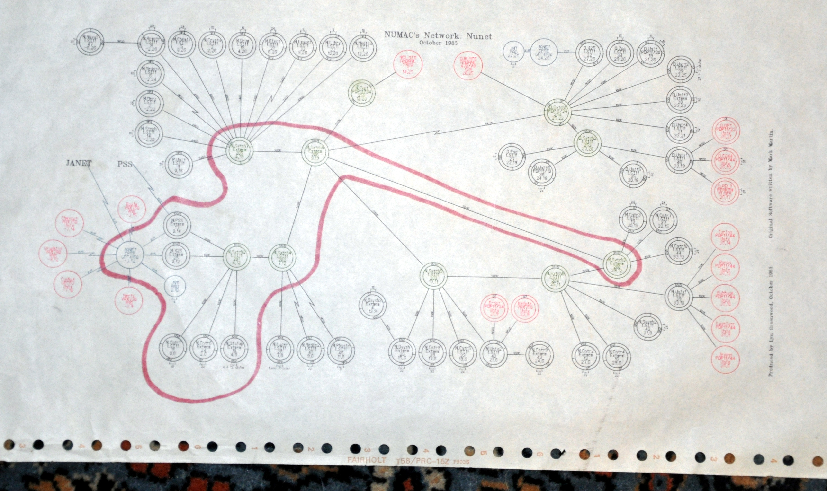
Durham campus network is in the top right quadrant, Newcastle in the other three. I have forgotten what the red felt tip encircled. I'll not say much about this diagram except that at the core were Swtchs that nodes connected to. Terminals connected to the nodes and users of the computing service sat at terminals using the interactive service provided by many computers coloured RED in the diagram, as envisaged 20 years earlier by Ewan Page.

In 1986 the Ethernet began to be introduced and would eventually replace NUNET.

Here is a network diagram from 1988:

Its size is 100cm by 40cm and here and there it is faded. By clicking on the image you can bring up the fullsize 6480pixel by 2792pixel, (it is two photos joined) 5.48MB image and scroll around it using the scroll bars. Where you will find:

• 12 [9] Switches (the figures in brackets are the 1985 count)
• 67 [43] Nodes. These are all DEC LSI11s computers except a couple of DEC PDP11s.
• 12 [3] Gateways. These connected NUNET to other networks that used different protocols.
• 13 [17] Service Computers. The computers the users were connecting to via the network.

Because of the difficulty of reading the diagram here is linear text version.

7 years later the network is transformed in 1995. The last mainframe went in 1992 and there is no mention of NUNET.

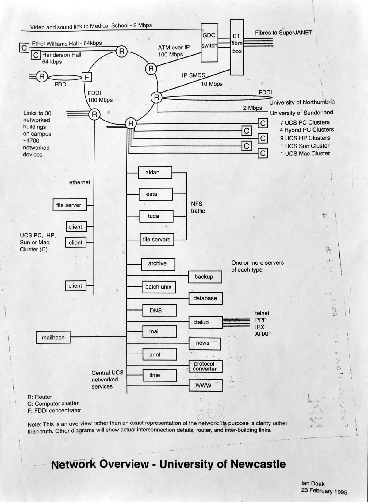
The heart of the network is the circle labelled FDDI 100Mbps (Fibre Distributed Data Interface).

Routers and Concentrators connect to the FDDI loop, connected to them is 10Mbps fibre Etthernet. One ethernet connected the central UCS (University Computing Service) servers. aidan, eata and tuda (Bishops of Lindisfarne on Holy Island) were general purpose Unix servers. To the same router was connected 22 clusters, numbering 10-30 machines, that were scattered around the campus at which students could log on to any and have access to their files and email. The network of a typical cluster can be seen to left of servers ethernet.

There were connections to the Universties of Northumbria and Sunderland because the Universty of Newcastle was the North East connection point to JANET (Joint Academic NETwork) that connected academic and research institutions in the UK

This next diagram is of JANET

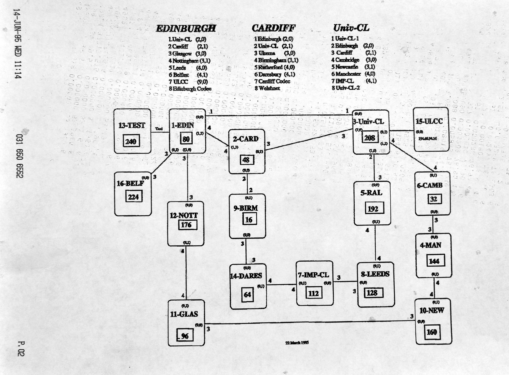
This again is 1995 drawn 22nd March and printed 14th June 1995.

It shows the backbone of JANET and at its core University College London, University of Edinburgh and Cardiff University. Connected to this core are two rings: Cambridge, Manchester, Newcastle, Glasgow and Nottigham; and Rutherford Appleton Labs, Leeds, Imperial Collage, Daresbury Laboratory and Birmingham. Belfast and University London Computing Centre were singly connected. Most institutions were thus doubly connected so able to survive a single link failure.

I do not know what all the numbers are.

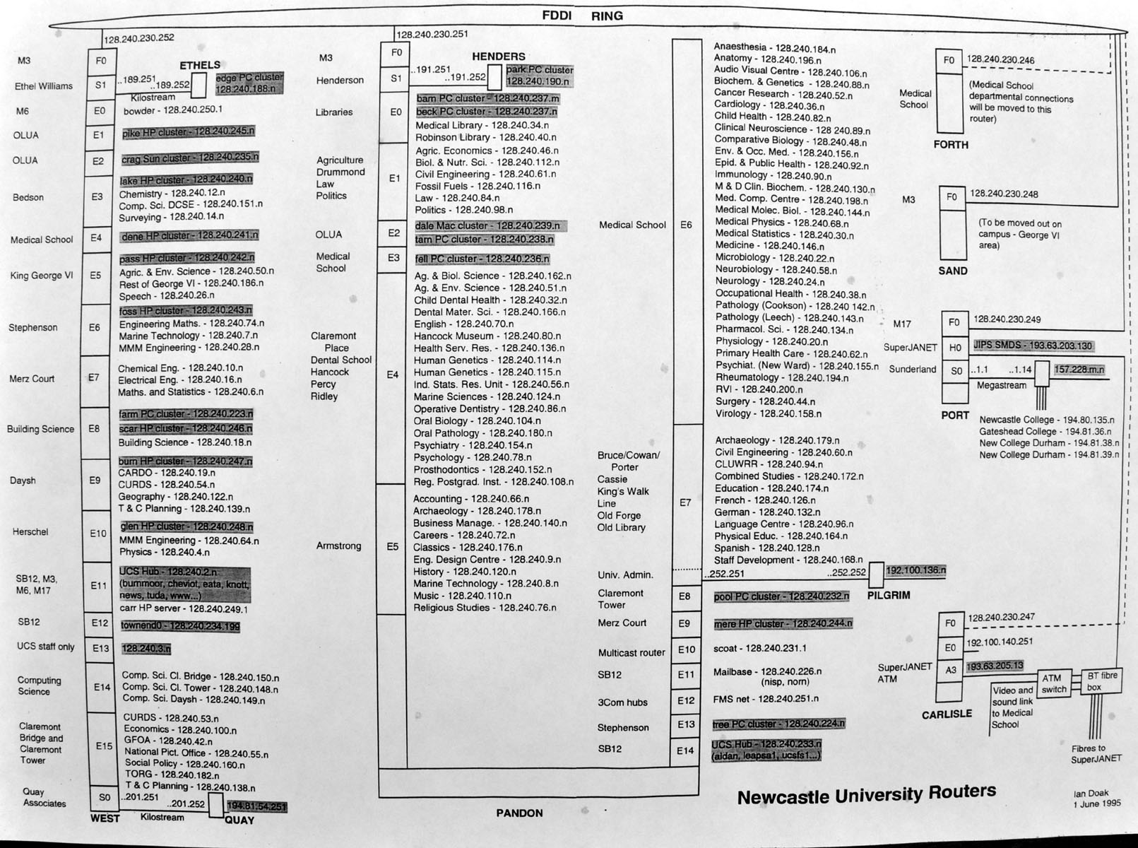
This diagram is entitled Newcastle University Routers.

Routers were very fast boxes connected to a very fast network that looked at every packet arriving and ignored it or routed it to a slower subnet that was connected to it. This meant that you did not need expensive very fast network everywhere. The slow subnet only had to carry its local traffic.

At the top is the FDDI loop and to it is connected routers. This diagram shows how the address space was allocated.

At this time internet addresses were IPv4 (Internet Protocol version 4) which were four bytes w.x.y.z where each could range from 0 - 255. This provided for 4294 million addresses. (As I write this in 2013 this IPv4 address space is exhauhsted and the Internet is using IPv6.)

Newcastle University was allocated 128.240.y.z. The Newcastle address space was subdivided by y=0-255 subnets and z=0-255 devices on each subnet. This diagram shows how the subnets were allocated and that the routers only had to inspect the "y" and "z" in the packet destination address to route the packet to one of its ports or ignore it.

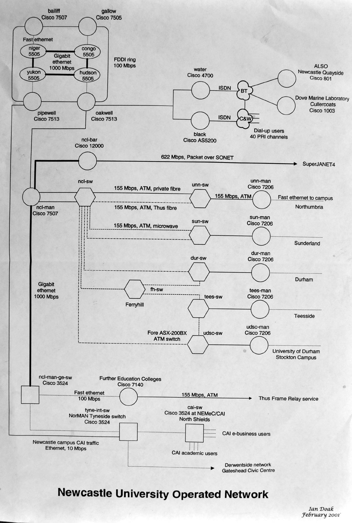
This network diagram entitled Newcastle University Operated Network dated February 2001.

It is a diagram of WAN (Wide Area Network) covering the North East of England.